Introduction to Changepoint Analysis
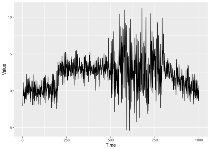
Having spent 3 years of my life studying changepoints in my PhD, I would hope I’d be able to succinctly overview the topic … lets see how it goes. First things first, the word changepoint can be spelt in many different ways (changepoint, change-point or change point) and if your looking in the economic literature they can also be called structural breaks - don’t be confused these are all describing the exact same thing!
Introduction
Changepoint analysis is exactly what it says on the tin; looking for points of change in ordered data. Time series data is the most common example of ordered data, although there are others such as the position along a genome in genetic applications. Figure 1 shows a collection of different time series containing different changepoints.
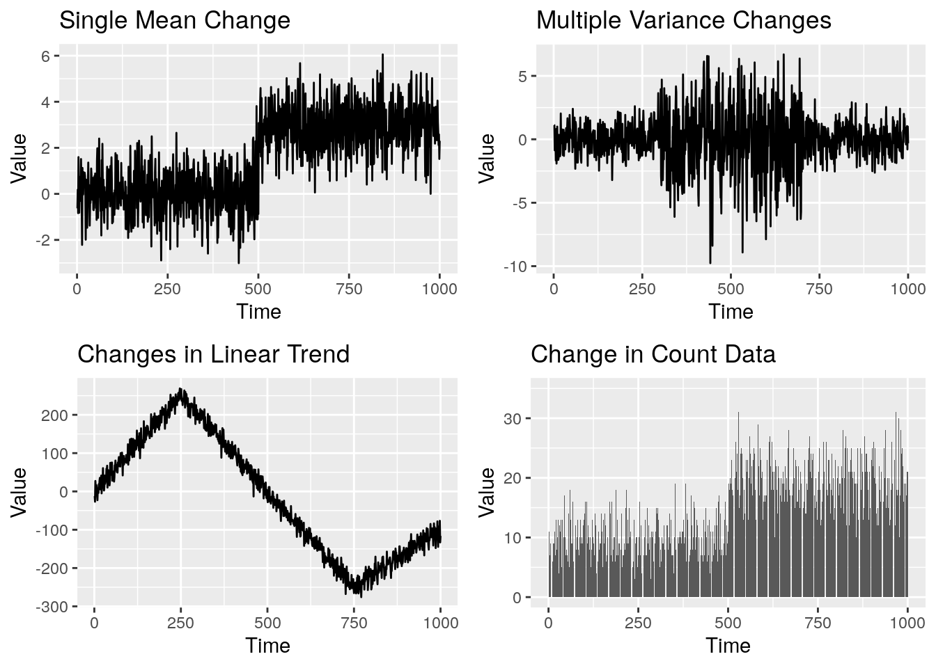
Figure 1: Examples of time series containing different changepoints
The aim of changepoint analysis is two-fold:
- Determine the number of changes in a series.
- Identify the position of the changes within the series.
Determining the number and location of the changepoints yields a segmentation of the data. A successful changepoint analysis will result in each segment being structurally similar (think having the same mean/variance/trend). In more technical language, we desire each segment to be stationary so the segmentation creates a piecewise stationary series. Technically, data with a trend isn’t stationary, however, we can easily make it stationary by differencing the data.
Finding Changepoints
Figure 1 showed some different types of changepoints. To keep things simple, we consider a single change in mean as shown in Figure 2 below.
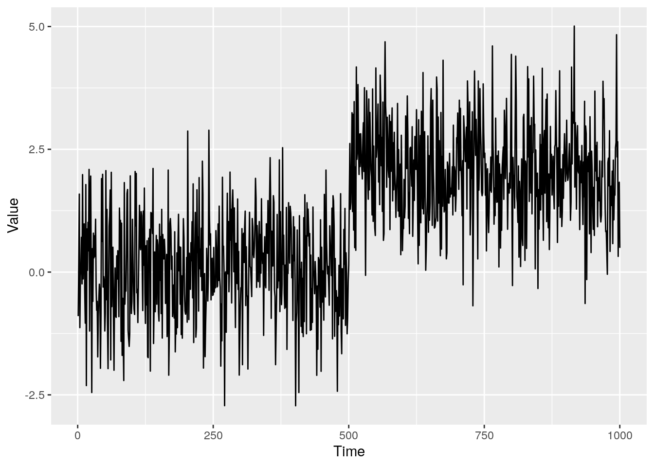
Figure 2: A single mean change in standard Guassian data
Looking at this plot, you can instantly see the location of the changepoint and the number of changes. So what’s the point in decades worth of research into a subject area that we can do instantly just by looking at the data? Well firstly, this is the most obvious type of changepoint, in more complicated examples it is not so easy to simply spot the changepoints by eye. Take a look at Figure 3, this a multivariate time series but can you spot the changepoint? I would be mightily impressed if you could! (p.s. the change is at 400 and is a change in covariance). Secondly, back to the simple change in mean scenario, what if I now gave you 10000 time series to look at and asked you to tell me where all the changepoints were? If you were rich enough you could hire 10000 people and get the answers instantly or you could utilize changepoint analysis. I’m going to assume we want to do the latter.
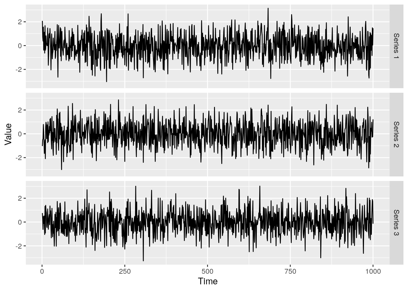
Figure 3: A multivarite time series with a change in covariance. Can you spot the changepoint by eye?
For the single change in mean scenario, we want our changepoint analysis to replicate what the human eye can do instantly - spot the change. How does your eye know where the change is though? If we break it down your eye is drawn to the point where the data jumps, but how does your eye know there is a jump? Well it can see the data points are first centered around 0 and then they are centered around 2. This, in essence, is noticing the mean of the time points has changed. This idea forms the basis of the most common changepoint method, the CUmulative SUM (CUSUM) method.
CUSUM
In simple changepoint examples, what makes the human eye the best changepoint detector in the world is it’s ability to instantly locate the change. Unfortunately, creating an algorithm that can just instantly spot a change isn’t possible (yet), so we have to break the problem down.
Imagine we had an incredibly long time series and its plot covered the length of a football pitch. How would you go about finding the change by eye? It’s not possible to view the whole series at once, so a sensible choice would be to start at one end and walk along until we came to the changepoint. In principle, this is exactly how we code changepoint algorithms. The basics of the CUSUM method is to start at one end of the data, calculate the mean before and after the time point and keep repeating this for each time point as we move through the data. The point where the difference between the means is the greatest is then our changepoint location.
To define the CUSUM statistic formally, we first need some basic notation. Let \(X_t\) be our data for \(t=1,\ldots,n\), where \(n\) is the length of the data. Let \(k\) be the point at which we split the data. The CUSUM test statistic, \(\text{CUSUM}(k)\), at point \(k\) is defined as \[ \text{CUSUM}(k)=\sqrt{\frac{k(n-k)}{n}}\left|\frac{1}{k}\sum\limits_{t=1}^kX_t-\frac{1}{n-k}\sum\limits_{t=k+1}^nX_t\right|\;.\]
Notice, the CUSUM statistic is actually a weighted difference of the means. This is to account for the size of the segment before and after \(k\). If we have less data, our estimate of the mean will be poorer and this is accounted for in the weighting.
So how does this CUSUM statistic behave with the single mean change in Figure 2? Below, Figure 4 shows the raw data and the CUSUM statistic at each point \(k\).
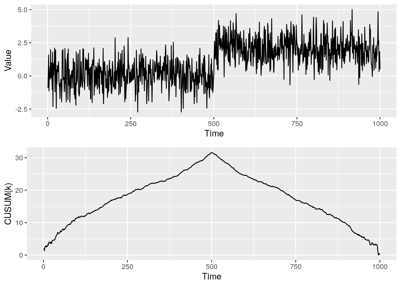
Figure 4: Single change in mean with the associated CUSUM statistic
We can see the CUSUM statistic is maximized at the changepoint location. Bingo! Hence, we choose our changepoint estimate, \(\hat{\tau}\), as the point which maximizes the CUSUM statistic, \[ \hat{\tau}=\max\limits_{1\leq k\leq n-1}\text{CUSUM}(k)\;. \] Okay so we’re finished right? We can now use the CUSUM statistic to find a single change in mean in our own data. Unfortunatley, we’re not quite there. If we think back to the main aims of changepoint analysis we’ve actually only answered one of them; we’ve located the position of the changepoint. We haven’t determined the number of changepoints, we just assumed there is 1 changepoint in the data. In reality, it is rare to know the exact number of changepoints. Instead, there are usually two scenarios:
- AMOC: This stands for At Most One Changepoint. I.e we know there is either one or zero changepoints in the data.
- Multiple Changepoints: The number of changepoints is completely unknown.
For now we focus on the AMOC setting, however, it can be relatively straightforward to extended methods designed for the AMOC setting to the multiple changepoint setting - look up Binary Segmentation to learn more.
AMOC scenario
The AMOC scenario has two options, none or one changepoint in the data. Figure 4 shows what the CUSUM statistic looks like if there is one changepoints, so lets see what it looks like for no changepoints. To make wording easier, we will refer to data containing no changepoints as null data and the data containing a changepoint as alternative data.
Figure 5 shows null data and the corresponding CUSUM statistic.
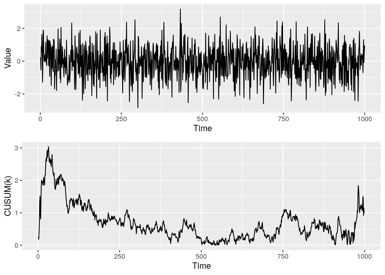
Figure 5: Series with no changepoints and the associated CUSUM statistic
What are the main differences between the CUSUM statistics for the null and alternative data? Well, for the alternative data the CUSUM statistic rises, almost linearly, to the maximum point at the changepoint location and then decreases, again almost linearly. On the other hand, for the null data, we see the CUSUM statistic is more random, we have an initial peak (this would be our estimated changepoint location) and then it fluctuates.
However, the main difference is revealed if we plot both the CUSUM statistics on the same plot. Figure 6 shows the two CUSUM statistics overlaid on each other.
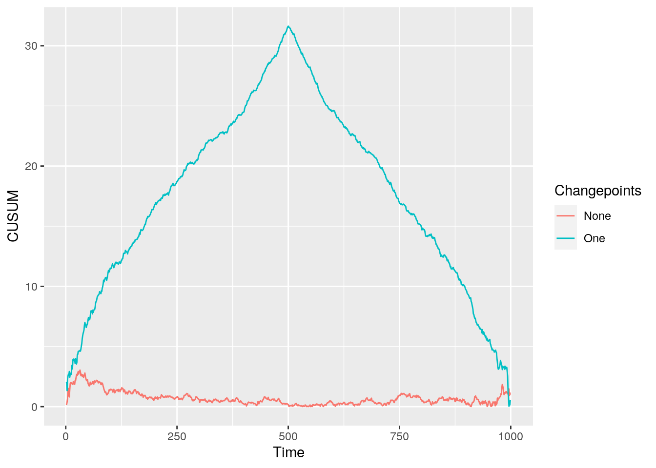
Figure 6: CUSUM statistic for data with none and a single changepoint
The main difference between the CUSUM statistics is now more obvious. For the alternative data the maximum CUSUM statistic is much larger than the CUSUM statistic for the null data. We can utilize this information to create a rule for determining if a changepoint has occurred. We deem a changepoint to be significant (i.e. a changepoint exists) if the maximum CUSUM statistic exceeds some threshold. But how do we choose a threshold?
Threshold Choice
Choosing an appropriate threshold is a challenging task and is usually problem specific. In general, we choose a threshold to control the false positive rate (FPR), also known as the type-1 error. This means if we had many series without a change, the proportion of series with a maximum CUSUM statistic exceeding the threshold is at most the FPR. So if we set our false positive rate at 5% then out of 500 series of null data we would expect to signal at most 25 as having a changepoint.
Lets simulate a threshold for our single mean change example. Note, we are assuming we know the distribution of the data before the change (in our examples it is \(N(0,1)\)) and we know the length of the data. To create a threshold we follow these steps:
- Create many series of data with no changepoints (here we use 500).
- Calculate the maximum CUSUM statistic for each series.
- Find the quantile that corresponds to the FPR we desire (here we set our FPR at 5% so find the 95% quantile).
Figure 7 shows a histogram of the maximum CUSUM statistics with our simulated threshold.
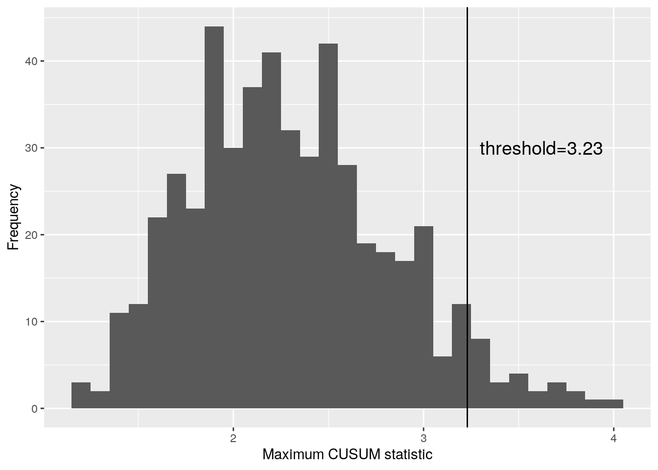
Figure 7: Histogram of maximum CUSUM statisitcs for data without a changepoint
Using this simulated threshold, Figure 8 shows the CUSUM statistics for the data with and without a change plus the threshold level of 3.23.
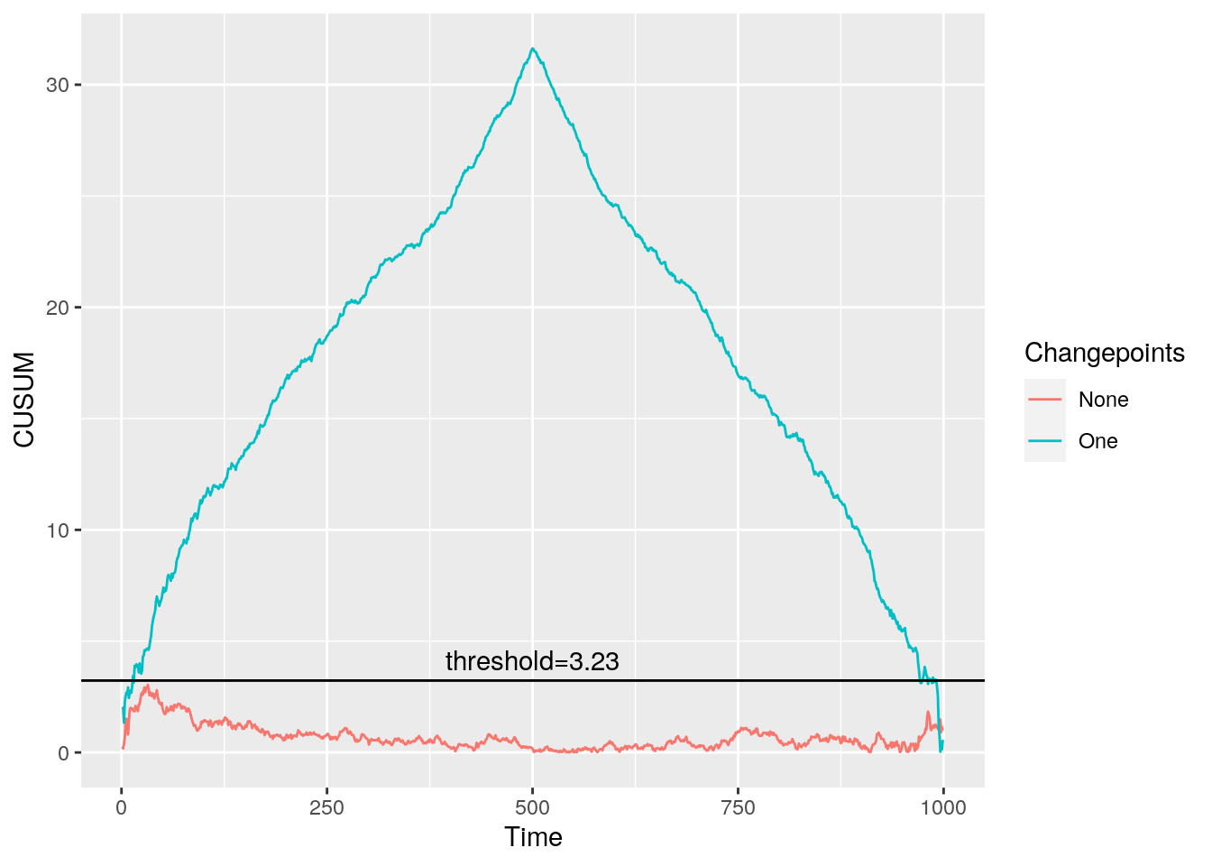
Figure 8: CUSUM statistic for data with none and a single changepoint with a simualted threshold
This threshold is performing as we would like. The CUSUM statistic for the data with a change is exceeding the threshold while the data without a change has a CUSUM statistic which stays below the threshold.
As noted above, to generate this threshold we required knowledge of the pre-change distribution of the data. In reality, this is rarely known and hence other techniques are need to generate a threshold.
Summary
So whats have we covered so far?
- Seen what changepoints look like in ordered data.
- Discussed the aims of changepoint analysis.
- Discovered a simple changepoint method for detecting mean changes.
- Explored how to determine if a data contains a changepoint or not using a threshold.
Hopefully, from this post you now understand the basics of changepoint analysis and could use the CUSUM statistic to identify changes in mean. There are many extensions in the changepoint literature which I haven’t had time to discuss here including:
- Detecting different types of changes (e.g. variance, trends, distributional).
- Alternative methods to the CUSUM (e.g. Likelihood Ratio Test).
- Identifying multiple changepoints.
- Detecting changepoints in multivariate data.
- Detecting changepoint sequentially, in an online fashion.
Who knows, I may get around to talking about some of them in later posts.